Quick-start guide: coupling with CPL Library
The aim of the following text is to lead the user, by example, from downloading CPL library, all the way through to running and analysing a coupled simulation. Please get in touch if something is unclear.Guide contents:
- Five Minute Quickstart
- Pre-requisites
- Download
- Compilation
- Demo: a minimal linking example
- Demo: a minimum send/recv example
- CPL Mocks
- Demo: visualising a coupled simulation
- Demo: Interactive GUI using CPL library
- Minimal CFD and MD code with coupling
Five Minute Quickstart
Assuming you use Docker, the easiest way to try out CPL library on your local linux computer is with the following command,
I don't use Docker
If you don't use Docker, or prefer not to, CPL library should be fairly easy to install on a unix based system, add the Pre-requisites and then follow the install instructions in the download and compilation sections. Make sure /lib/libcpl.so exists and you have called
In the Docker container (or installed CPL library folder), change directory to the examples,
These examples show the minimal code needed to run a coupled simulation in the three supported languages, Fortran, C++ and Python. Have a look at the code in these files, you will see the CPL_init, CPL_setup, CPL_send and CPL_recv commands, as well as boilerplate to setup MPI and create a cartesian topology. You can compile the Fortran code using,
for the C++ code, you compile using,
Both cplf90 and cplc++ are just wrappers for mpif90 and mpic++ respectively, including all the shared libraries and included needed for coupling (see Compilation. A coupled run is then performed using,
This will run each executable on one processes and link them together, exchanging information using MPI and printing to screen the output from both codes. Similarly, the other Python
or the other Fortran or C++ codes could be compiled and used instead.
The runner cplexec is simply a Python wrapper which runs both excutables as separate MPI
processes with their own MPI_COMM_WORLDS, which are then linked together using MPI Port.
Alternatively, the two executables can be run in Multiple Processes Multiple Data (MPMD) mode,
using,
where both codes share a single MPI_COMM_WORLD.
That's it, this example contains the basic premise of CPL library, run two codes, link them together, setup a topological mapping and exchange information. Next step can be to adjust the input parameter in any of the dummy codes to see what happens, run with different numbers of processes by adjusting the input values in both codes or try changing the coupler input file COUPLER.in.
Once you understand the way CPL library links two any executables in Fortran, C++ or Python and exchanges information through CPL send and CPL recv, you can move on to the other examples. The interactive examples may need display setup in Docker, see the extended documentation. You can then look into OpenFOAM and LAMMPS coupling,
And check out the examples in cpl-library/examples/coupled, as well as test folders in the two coupling APPS, /CPL_APP_LAMMPS-DEV, here and /OpenFOAM/CPL_APP_OPENFOAM-3.0.1 here. The APPS use the minimal dummy scripts above like mocks to test coupling and develop new code. Combined with assert statements and testing functions, it is possible to build up a range of automated tests for coupled codes to divide and validate a coupled simulation. This is the recommended way to develop new coupled cases and the first case you should aim to get running. By dividing the problem into a mock script and one of the coupled codes, you can control exactly what is sent and plot returned values to make sure each code behaves correctly by itself.
Pre-requisites
Before you begin installing CPL library either locally or on your supercomputer, make sure you have the following installed on your system:- A Fortran compiler that supports the F2008 standard
- A C/C++ compiler that supports the C++11 standard
- An MPI library - currently MPICH is recommended but OpenMPI is supported
IMPORTANT NOTE: To minimise compatibility problems,
you are advised to install gcc-5 and gfortran-5 or later
(from a ppa or build it yourself).
If you have a modern linux distribution (e.g. 16.04 or later)
then MPICH can also be got from a ppa (be sure to remove or switch
from any existing OpenMPI installations).
On older systems, it may be best to download the latest version of MPICH and
build this new version with a version of gcc and gfortran later than 5.
MPICH with gcc-5 setup
/PATH/TO/INSTALL/mpich_gcc5/ \
CXX=gcc-5 FC=gfortran-5
$make
$make install
$ export PATH:/PATH/TO/INSTALL/mpich_gcc5/:$PATH
For testing and visualisation, you will optionally need a range of Python tools, these include,
- The following packages for Python2.7 from a package manager: python-dev, python-pip, python-tk and python-wxgtk3.0,
- From pip, install matplotlib, numpy, scipy, pytest and mpi4py (ensure mpi4py is using the same MPI as CPL library and all other coupled codes)
Download
To keep up-to-date with bug-fixes and future developments, the user is encouraged to download the git version:
$ git clone https://github.com/Crompulence/cpl-library.git
If you don't want to use git, You can also download from github as a zip file,
https://github.com/Crompulence/cpl-library/archive/master.zip
Then unzip the file and rename the folder to "cpl-library":Compilation
Compiling CPL library itself, as a shared library, is likely to work with a single make command:
The platform commands specifies the platform specific options, a list of which are available in the cpl-library/make folder. This build has been verified for the GCC compiler collection and MPICH. Support for Intel (R) compiler suites have also been tested on various platforms. For more specific build requirements, the user should copy and change the compiler template file as outlined in cpl-library/README. Note that CPL library is not installed. Instead, a library will be created at the path,
C++ headers and Fortran use-modules are placed in
The wrapper scripts for cplf90, cplc++ and cplexec are located in
These can be added to the user's path by calling,
which can be added to the user .bashrc if desired, and is preferred to installing into the system directory as different versions of CPL library may be used with different version of MPI or compilers. Note, a make install option is provided but has not been fully tested for all versions of linux.
Demo: a minimal linking example
All examples are all included in the /cpl-library/examples folder with the CPL library software.
This simple example shows you how to link two massively-parallel codes with CPL library. The example MD code is written in Fortran, and the CFD code in C++. Both programs may run with any number of processes. Take a look at the simple Fortran example code:
program main_MD
   use cpl, only : CPL_init, CPL_finalize
   use mpi
   implicit none

   integer :: rank, nprocs, ierr
   integer :: MD_COMM
   integer, parameter :: MD_realm=2

   !Initialise MPI
   call MPI_Init(ierr)

   !Create MD Comm by spliting world
   call CPL_init(MD_realm, MD_COMM, ierr)

   call MPI_comm_size(MD_COMM, nprocs, ierr)
   call MPI_comm_rank(MD_COMM, rank, ierr)

   print*, "MD code processor ", rank+1, " of ", nprocs

   !No need for seperate CPL finalise as MPI finalise takes care of this
   call CPL_finalize(ierr)
   call MPI_comm_free(MD_COMM,ierr)
   call MPI_finalize(ierr)

end program main_MD
This code initialises MPI, and gets the MD communicator from CPL library. It must, therefore, be linked to both the MPI and CPL libraries when it is compiled. The compilation can be performed with a call to mpif90 of the form:
-I${CPL_PATH}/include/cpl \
-L${CPL_PATH}/lib \
-Wl,-rpath=${CPL_PATH}/lib/ \
-o ./mdProgram -lcpl
If you're not familiar with the processes involved in linking
shared libraries to software, there are a few things to notice
in the above command.
The variable CPL_PATH should be set to the location of the base
directory of the CPL library downloaded,
unzipped and build in the previous section.
First, we've specified the location of the
Fortran module files with the -I flag.
Second, the location of the cpl-library shared library,
libcpl.so, is specified with -L.
Because the library is a dynamic one, not in the standard
/usr/lib location, we also provide the built
executable with a reference to the library location with
-Wl,-rpath=${CPL_PATH}/lib/.
Note: all compiler flags for the MPI library
are handled automatically by the mpic++ and
mpif90 compiler wrappers.
Two helper scripts similar to MPI are provided to simplify linking in
${CPL_PATH}/bin folder. These can be included in the path using,
Note if you want to specify the cpl path to a different directory than the location of SOURCEME.sh, you need to set
manually. After adding CPL library to your path with SOURCEME.sh, the previous build statement then simply becomes,
Next we build an equivalent CFD demo program written in C++:
#include "cpl.h"
#include "mpi.h"
#include <iostream>

using namespace std;

int main() {
   MPI_Init(NULL, NULL);

   int CFD_realm = 1;
   MPI_Comm CFD_COMM;
   CPL::init(CFD_realm, CFD_COMM);

   int nprocs; int rank;
   MPI_Comm_size(CFD_COMM, &nprocs);
   MPI_Comm_rank(CFD_COMM, &rank);

   cout << "MD code processor " << rank+1 << " of " << nprocs << endl;

   CPL::finalize();
   MPI_Finalize();
}
Like the Fortran example above, the compilation command is of the form:
-I${CPL_PATH}/include/cpl \
-L${CPL_PATH}/lib \
-Wl,-rpath=${CPL_PATH}/lib/ \
-o ./cfdProgram -lcpl
This time, the -I flag tells the compiler where to
find the CPL library C++ header files, and we must link to the
-lgfortran and -lmpifort Fortran libraries.
Alternativly using cplc++ wrapper,
Now the demo codes are compiled, they can be executed together in the run directory with:
That's it! The codes should execute, and CPL library will tell you that its internal communicators have been initialised. Obviously it is rarely that simple, if you get any problems, please check out the faq section and if this doesn't help, please get in touch.
The fortran code can also be easily replaced with a python example,
from mpi4py import MPI
from cplpy import CPL

comm = MPI.COMM_WORLD
CPL = CPL()
MD_COMM = CPL.init(CPL.MD_REALM)

nprocs = MD_COMM.Get_size()
rank = MD_COMM.Get_rank()

print(("MD code processor "+ str(rank+1) + " of " + str(nprocs)))

CPL.finalize()
MPI.Finalize()
there is no need to compile, but the path must be correctly set. This can also be done using,
if you haven't already. SOURCEME.sh appends the library location and python ctype bindings to the PYTHONPATH variable. A python and C++ coupled example can then be run using,
These examples don't actually do anything interesting, and so in the next section, the minimal code is presented to send and recieve data.
Demo: a minimum send/recv example
This section outlines a first and simplest example of coupling. An array of cells with three components per cell is packed with the x, y and z global index of the cell, shown here for 2D indices only,
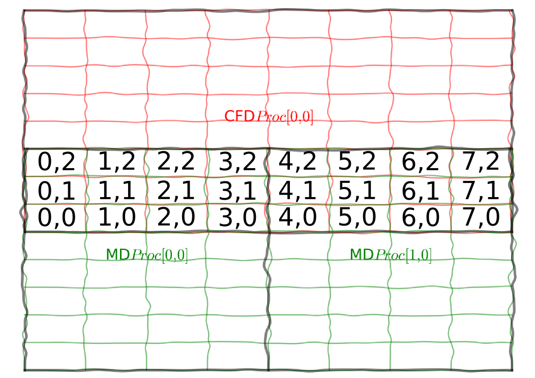
This is sent, from CFD to MD and checked. Although this isn't the most exciting example, it does provide a clear picture of exactly how CPL library works. The global system of cells is setup and split over many processors in both the MD and CFD codes. The coupled simulation has some overlap, specified in the COUPLER.in file in the cpl folder. This determines how the two codes overlap and the topological relationship between them. The mapping of processors is handled by CPL library using a minimal set of inputs. First, initialisation is performed with a call to CPL_init. This splits MPI_COMM_WORLD into two MPI communicators for the MD and CFD realms. The grid information and topological mapping is performed using calls to CPL_setup_md on the MD side and CPL_setup_cfd for the CFD. The CPL_send and CPL_recv functions then exchange all information for the grid in the overlap region with all information exchanged only between processes that are topological overlapping. This avoids any global communications and maintains the scaling of the two codes. The send/recv limits are specified in global grid coordinates and should be consistent between codes. This means the user does not need to know about the processor topology of the two codes. The examples in this section start with fortran, then c++ and finally python.
Fortran
This section outlines a minimal example in Fortan which will send information between an MD and CFD code.
The CFD code is first,
See CFD Fortran Code
program cfd_cpl_example
    use cpl, only : CPL_init, CPL_setup_cfd, &
                    CPL_get_olap_limits, CPL_my_proc_portion, &
                    CPL_get_no_cells, CPL_send, CPL_recv, &
                    CPL_finalize
    use mpi
    implicit none

    logical :: recv_flag, send_flag, NO_ERROR
    integer :: i,j,k,ii,jj,kk,ierr
    integer :: NPx, NPy, NPz, NProcs, rank
    integer :: nprocs_realm
    integer :: CART_COMM, CFD_COMM
    integer, parameter :: cfd_realm=1
    integer, dimension(3) :: npxyz, Ncells, ncxyz
    integer, dimension(6) :: portion, limits
    double precision, dimension(3)  :: xyzL, xyz_orig
    double precision, dimension(:,:,:,:), &
         allocatable  :: send_array

    !Initialise MPI
    call MPI_Init(ierr)

    !Create MD Comm by spliting world
    call CPL_init(CFD_realm, CFD_COMM, ierr)

    ! Parameters of the cpu topology (cartesian grid)
    xyzL = (/10.d0, 10.d0, 10.d0/)
    xyz_orig = (/0.d0, 0.d0, 0.d0/)
    npxyz = (/ 2, 2, 1/)
    ncxyz = (/ 64, 18, 64 /)

    ! Create communicators and check that number of processors is consistent
    call MPI_Comm_size(CFD_COMM, nprocs_realm, ierr)
    if (nprocs_realm .ne. product(npxyz)) then
        print'(4(a,i6))', "Non-coherent number of processes in CFD ", nprocs_realm, &
                " no equal to ",  npxyz(1), " X ", npxyz(2), " X ", npxyz(3)
        call MPI_Abort(MPI_COMM_WORLD, 1, ierr)
    endif

    !Setup cartesian topology
    call MPI_comm_rank(CFD_COMM, rank, ierr)
    call MPI_Cart_create(CFD_COMM, 3, npxyz, (/.true., .true., .true./), &
                         .true., CART_COMM, ierr)

    !Coupler setup
    call CPL_setup_cfd(CART_COMM, xyzL, xyz_orig, ncxyz)

    !Get detail for grid
    call CPL_get_olap_limits(limits)
    call CPL_my_proc_portion(limits, portion)
    call CPL_get_no_cells(portion, Ncells)

    ! Pack send_array with cell coordinates. Each cell in the array carries
    ! its global cell number within the overlap region.
    allocate(send_array(3, Ncells(1), Ncells(2), Ncells(3)))
    do i = 1,Ncells(1)
    do j = 1,Ncells(2)
    do k = 1,Ncells(3)
        ! -2 indices to match c++ and python indexing in portion and i,j,k
        ii = i + portion(1) - 2
        jj = j + portion(3) - 2
        kk = k + portion(5) - 2

        send_array(1,i,j,k) = ii
        send_array(2,i,j,k) = jj
        send_array(3,i,j,k) = kk
    enddo
    enddo
    enddo

    call CPL_send(send_array, limits, send_flag)

    !Block before checking if successful
    call MPI_Barrier(MPI_COMM_WORLD, ierr)

    !Release all coupler comms
    call CPL_finalize(ierr)

    !Deallocate arrays, free comms and finalise MPI
    deallocate(send_array)
    call MPI_Comm_free(CFD_COMM, ierr)
    call MPI_Comm_free(CART_COMM, ierr)
    call MPI_finalize(ierr)

end program cfd_cpl_example
Now the MD code which receives data from the CFD code and
See MD Fortran Code
program md_cpl_example
    use cpl, only : CPL_init, CPL_setup_md, &
                    CPL_get_olap_limits, CPL_my_proc_portion, &
                    CPL_get_no_cells, CPL_send, CPL_recv, &
                    CPL_overlap, CPL_finalize
    use mpi
    implicit none

    logical :: recv_flag,send_flag, NO_ERROR
    integer :: i,j,k,ii,jj,kk,ierr,errorcode
    integer :: rank, nprocs_realm
    integer :: CART_COMM, MD_COMM
    integer, parameter :: md_realm=2
    integer, dimension(3) :: npxyz, Ncells
    integer, dimension(6) :: portion, limits
    double precision, dimension(3)  :: xyzL, xyz_orig
    double precision, dimension(:,:,:,:), allocatable  :: recv_array, send_array

    !Initialise MPI
    call MPI_Init(ierr)

    !Create MD Comm by spliting world
    call CPL_init(md_realm, MD_COMM, ierr)

    ! Parameters of the cpu topology (cartesian grid)
    xyzL = (/10.d0, 10.d0, 10.d0/)
    xyz_orig = (/0.d0, 0.d0, 0.d0/)
    npxyz = (/ 4, 2, 2/)

    ! Create communicators and check that number of processors is consistent
    call MPI_Comm_size(MD_COMM, nprocs_realm, ierr)

    if (nprocs_realm .ne. product(npxyz)) then
        print'(4(a,i6))', "Non-coherent number of processes in MD ", nprocs_realm, &
                " no equal to ",  npxyz(1), " X ", npxyz(2), " X ", npxyz(3)
        call MPI_Abort(MPI_COMM_WORLD, errorcode, ierr)
    endif

    !Setup cartesian topology
    call MPI_comm_rank(MD_COMM, rank, ierr)
    call MPI_Cart_create(MD_COMM, 3, npxyz, (/.true.,.true.,.true./), &
                         .true., CART_COMM, ierr)

    !Coupler setup
    call CPL_setup_md(CART_COMM, xyzL, xyz_orig)

    !Get detail for grid
    call CPL_get_olap_limits(limits)
    call CPL_my_proc_portion(limits, portion)
    call CPL_get_no_cells(portion, Ncells)

    !Coupled Recieve and print
    allocate(recv_array(3, Ncells(1), Ncells(2), Ncells(3)))
    recv_array = 0.d0
    call CPL_recv(recv_array, limits, recv_flag)

    ! Check that every processor inside the overlap region receives the cell correctly
    ! number.
    if (CPL_overlap()) then
        no_error = .true.
        do i = 1, Ncells(1)
        do j = 1, Ncells(2)
        do k = 1, Ncells(3)
            ! -2 indices to match c++ and python indexing in portion and i,j,k
            ii = i + portion(1) - 2
            jj = j + portion(3) - 2
            kk = k + portion(5) - 2

            if ((dble(ii) - recv_array(1,i,j,k)) .gt. 1e-8) then
                print'(a,2i5,a,i5,a,i6,a,f10.5)', "ERROR -- portion in x: ", portion(1:2), &
                       " MD rank: ", rank, " cell i: ",ii, &
                       " recv_array: ", recv_array(1,i,j,k)
                no_error = .false.
            endif
            if ((dble(jj) - recv_array(2,i,j,k)) .gt. 1e-8) then
                print'(a,2i5,a,i5,a,i6,a,f10.5)', "ERROR -- portion in y: ", portion(3:4), &
                       " MD rank: ", rank, " cell j: ", jj , &
                       " recv_array: ", recv_array(2,i,j,k)
                no_error = .false.
            endif
            if ((dble(kk) - recv_array(3,i,j,k)) .gt. 1e-8) then
                print'(a,2i5,a,i5,a,i6,a,f10.5)', "ERROR -- portion in z: ", portion(5:6), &
                       " MD rank: ", rank, " cell k: ", kk , &
                       " recv_array: ", recv_array(3,i,j,k)
                no_error = .false.
            endif
        enddo
        enddo
        enddo
    endif

    !Block before checking if successful
    call MPI_Barrier(MD_COMM, ierr)
    if (CPL_overlap() .and. no_error) then
        print'(a,a,i2,a)', "MD -- ", "(rank=", rank, ") CELLS HAVE BEEN RECEIVED CORRECTLY."
    endif
    call MPI_Barrier(MPI_COMM_WORLD, ierr)

    !Release all coupler comms
    call CPL_finalize(ierr)

    !Deallocate arrays and finalise MPI
    deallocate(recv_array)
    call MPI_Comm_free(MD_COMM, ierr)
    call MPI_Comm_free(CART_COMM, ierr)
    call MPI_finalize(ierr)

end program
This can be built using,
and similar for cfd executable,
and run using
The coupled simulation sends data from the 16 MD processors to the 4 CFD processors. These are then checked to ensure they correspond the correct locations in space and any errors are printed. A correct output will contain something like,
MD -- (rank= 3) CELLS HAVE BEEN RECEIVED CORRECTLY.
MD -- (rank= 6) CELLS HAVE BEEN RECEIVED CORRECTLY.
MD -- (rank= 7) CELLS HAVE BEEN RECEIVED CORRECTLY.
MD -- (rank=10) CELLS HAVE BEEN RECEIVED CORRECTLY.
MD -- (rank=11) CELLS HAVE BEEN RECEIVED CORRECTLY.
MD -- (rank=14) CELLS HAVE BEEN RECEIVED CORRECTLY.
MD -- (rank=15) CELLS HAVE BEEN RECEIVED CORRECTLY.
The examples for C++ and python are included next.
C++
This section outlines a minimal example in C++ which will send information between an MD and CFD code. The C bindings are similar.
See CFD C++ code
#include "mpi.h"
#include <iostream>

#include "cpl.h"
#include "CPL_ndArray.h"

using namespace std;

int main() {
   MPI_Init(NULL, NULL);

   int CFD_realm = 1;
   MPI_Comm CFD_COMM;
   CPL::init(CFD_realm, CFD_COMM);

   // Parameters of the cpu topology (cartesian grid)
   double xyzL[3] = {10.0, 10.0, 10.0};
   double xyz_orig[3] = {0.0, 0.0, 0.0};
   int npxyz[3] = {2, 2, 1};
   int ncxyz[3] = {64, 18, 64};

   int nprocs_realm;
   MPI_Comm_size(CFD_COMM, &nprocs_realm);

   // Create communicators and check that number of processors is consistent
   if (nprocs_realm != (npxyz[0] * npxyz[1] * npxyz[2])) {
      cout << "Non-coherent number of processes." << endl;
      MPI_Abort(MPI_COMM_WORLD, 1);
   }

   // Setup cartesian topology
   int rank;
   MPI_Comm_rank(CFD_COMM, &rank);
   int periods[3] = {1, 1, 1};
   MPI_Comm CART_COMM;
   MPI_Cart_create(CFD_COMM, 3, npxyz, periods, 1, &CART_COMM);

   // Coupler setup
   CPL::setup_cfd(CART_COMM, xyzL, xyz_orig, ncxyz);

   // Get detail for grid
   int Ncells[3];
   int olap_limits[6], portion[6];
   CPL::get_olap_limits(olap_limits);
   CPL::my_proc_portion(olap_limits, portion);
   CPL::get_no_cells(portion, Ncells);

   // Pack send_array with cell coordinates. Each cell in the array carries
   // its global cell number within the overlap region.
   int send_shape[4] = {3, Ncells[0], Ncells[1], Ncells[2]};
   CPL::ndArray<double> send_array(4, send_shape);
   int ii, jj, kk;
   for (int i = 0; i < Ncells[0]; i++) {
       ii = i + portion[0];
       for (int j = 0; j < Ncells[1]; j++) {
           jj = j + portion[2];
           for (int k = 0; k < Ncells[2]; k++) {
               kk = k + portion[4];

               send_array(0, i, j, k) = (double) ii;
               send_array(1, i, j, k) = (double) jj;
               send_array(2, i, j, k) = (double) kk;
           }
        }
    }

   CPL::send(send_array.data(), send_array.shapeData(), olap_limits);

   // Block before checking if successful
   MPI_Barrier(MPI_COMM_WORLD);

   // Release all coupler comms
   CPL::finalize();
   MPI_Comm_free(&CFD_COMM);
   MPI_Comm_free(&CART_COMM);
   MPI_Finalize();

}
and the MD code,
See MD C++ code
#include "mpi.h"
#include <iostream>
#include <stdio.h>
#include <string>

#include "cpl.h"
#include "CPL_ndArray.h"

using namespace std;

int main() {
   MPI_Init(NULL, NULL);

   int MD_realm = 2;
   MPI_Comm MD_COMM;
   CPL::init(MD_realm, MD_COMM);

   // Parameters of the cpu topology (cartesian grid)
   double xyzL[3] = {10.0, 10.0, 10.0};
   double xyz_orig[3] = {0.0, 0.0, 0.0};
   int npxyz[3] = {4, 2, 2};

   int nprocs_realm;
   MPI_Comm_size(MD_COMM, &nprocs_realm);

   // Create communicators and check that number of processors is consistent
   if (nprocs_realm != (npxyz[0] * npxyz[1] * npxyz[2])) {
      cout << "Non-coherent number of processes." << endl;
      MPI_Abort(MPI_COMM_WORLD, 1);
   }

   // Setup cartesian topology
   int rank;
   MPI_Comm_rank(MD_COMM, &rank);
   int periods[3] = {1, 1, 1};
   MPI_Comm CART_COMM;
   MPI_Cart_create(MD_COMM, 3, npxyz, periods, true, &CART_COMM);

   // Coupler setup
   CPL::setup_md(CART_COMM, xyzL, xyz_orig);

   // Get detail for grid
   int Ncells[3];
   int olap_limits[6], portion[6];
   CPL::get_olap_limits(olap_limits);
   CPL::my_proc_portion(olap_limits, portion);
   CPL::get_no_cells(portion, Ncells);

   // Pack recv_array with cell coordinates. Each cell in the array carries
   // its global cell number within the overlap region.
   int recv_shape[4] = {3, Ncells[0], Ncells[1], Ncells[2]};
   CPL::ndArray<double> recv_array(4, recv_shape);
   CPL::recv(recv_array.data(), recv_array.shapeData(), olap_limits);
   bool no_error = true;
   if (CPL::overlap()) {
       int ii, jj, kk;
       for (int i = 0; i < Ncells[0]; i++) {
           ii = i + portion[0];
           for (int j = 0; j < Ncells[1]; j++) {
               jj = j + portion[2];
               for (int k = 0; k < Ncells[2]; k++) {
                   kk = k + portion[4];
                   if (((double) ii - recv_array(0, i, j, k)) > 1e-8) {
                       printf("Error -- portion in x: %d %d MD rank: %d cell i: %d recv_array: %f\n",\
                               portion[0], portion[1], rank, ii, recv_array(0, i, j, k));
                       no_error = false;
                   }
                   if (((double) jj - recv_array(1, i, j, k)) > 1e-8) {
                       printf("Error -- portion in y: %d %d MD rank: %d cell j: %d recv_array: %f\n",\
                               portion[2], portion[3], rank, jj, recv_array(1, i, j, k));
                       no_error = false;
                   }
                   if (((double) kk - recv_array(2, i, j, k)) > 1e-8) {
                       printf("Error -- portion in z: %d %d MD rank: %d cell k: %d recv_array: %f\n",\
                               portion[1], portion[5], rank, kk, recv_array(2, i, j, k));
                       no_error = false;
                   }
               }
            }
        }
    }

   // Block before checking if successful
   MPI_Barrier(MD_COMM);
   if (CPL::overlap() && no_error)
       printf("MD -- (rank=%2d) CELLS HAVE BEEN RECEIVED CORRECTLY.\n", rank);
   MPI_Barrier(MPI_COMM_WORLD);

   // Release all coupler comms
   CPL::finalize();
    MPI_Comm_free(&MD_COMM);
    MPI_Comm_free(&CART_COMM);
   MPI_Finalize();
}
python
This section outlines a minimal example in python which will send information between an MD and CFD code. The CFD code is first.
See CFD python Code
from mpi4py import MPI
from cplpy import CPL
import numpy as np

comm = MPI.COMM_WORLD
CPL = CPL()
nsteps = 1
dt = 0.2
density = 0.8

# Parameters of the cpu topology (cartesian grid)
NPx = 2
NPy = 2
NPz = 1
NProcs = NPx*NPy*NPz

# Parameters of the mesh topology (cartesian grid)
ncxyz = np.array([64, 18, 64], order='F', dtype=np.int32)
xyzL = np.array([10.0, 10.0, 10.0], order='F', dtype=np.float64)
xyz_orig = np.array([0.0, 0.0, 0.0], order='F', dtype=np.float64)

# Create communicators and check that number of processors is consistent
CFD_COMM = CPL.init(CPL.CFD_REALM)
nprocs_realm = CFD_COMM.Get_size()

if (nprocs_realm != NProcs):
    print("ERROR: Non-coherent number of processors.")
    comm.Abort(errorcode=1)

cart_comm = CFD_COMM.Create_cart([NPx, NPy, NPz])
CPL.setup_cfd(cart_comm, xyzL, xyz_orig, ncxyz)

cart_rank = cart_comm.Get_rank()
olap_limits = CPL.get_olap_limits()
portion = CPL.my_proc_portion(olap_limits)
[ncxl, ncyl, nczl] = CPL.get_no_cells(portion)
send_array = np.zeros((3, ncxl, ncyl, nczl), order='F', dtype=np.float64)

for i in range(0, ncxl):
    for j in range(0, ncyl):
        for k in range(0, nczl):
            ii = i + portion[0]
            jj = j + portion[2]
            kk = k + portion[4]

            send_array[0, i, j, k] = ii
            send_array[1, i, j, k] = jj
            send_array[2, i, j, k] = kk

ierr = CPL.send(send_array, olap_limits)

MPI.COMM_WORLD.Barrier()

CFD_COMM.Free()
cart_comm.Free()

CPL.finalize()
MPI.Finalize()
and the MD code,
See MD python Code
from mpi4py import MPI
from cplpy import CPL
import numpy as np


def read_input(filename):
    with open(filename, 'r') as f:
        content = f.read()

    dic = {}
    for i in content.split('\n'):
        if i.find("!") != -1:
            name = i.split("!")[1]
            value = i.split('!')[0].replace(' ', '')
            dic[name] = value
    return dic

comm = MPI.COMM_WORLD
#comm.Barrier()
CPL = CPL()

# Parameters of the cpu topology (cartesian grid)
dt = 0.1
NPx = 4
NPy = 2
NPz = 2
NProcs = NPx*NPy*NPz
npxyz = np.array([NPx, NPy, NPz], order='F', dtype=np.int32)

# Domain topology
xyzL = np.array([10.0, 10.0, 10.0], order='F', dtype=np.float64)
xyz_orig = np.array([0.0, 0.0, 0.0], order='F', dtype=np.float64)

# Create communicators and check that number of processors is consistent
MD_COMM = CPL.init(CPL.MD_REALM)
nprocs_realm = MD_COMM.Get_size()

if (nprocs_realm != NProcs):
    print("Non-coherent number of processes")
    comm.Abort(errorcode=1)

cart_comm = MD_COMM.Create_cart([NPx, NPy, NPz])

CPL.setup_md(cart_comm, xyzL, xyz_orig)

# recv test
olap_limits = CPL.get_olap_limits()
portion = CPL.my_proc_portion(olap_limits)
[ncxl, ncyl, nczl] = CPL.get_no_cells(portion)

recv_array = np.zeros((3, ncxl, ncyl, nczl), order='F', dtype=np.float64)
recv_array, ierr = CPL.recv(recv_array, olap_limits)

no_error = True
if CPL.overlap():
    rank = MD_COMM.Get_rank()
    for i in range(0, ncxl):
        for j in range(0, ncyl):
            for k in range(0, nczl):
                ii = i + portion[0]
                jj = j + portion[2]
                kk = k + portion[4]
                if (float(ii) - recv_array[0, i, j, k]) > 1e-8:
                    print("ERROR -- portion in x: %d %d " % (portion[0],
                          portion[1]) + " MD rank: %d " % rank +
                          " cell id: %d " % ii + " recv_array: %f" %
                          recv_array[0, i, j, k])
                    no_error = False

                if (float(jj) - recv_array[1, i, j, k]) > 1e-8:
                    print("ERROR -- portion in y: %d %d " % (portion[2],
                          portion[3]) + " MD rank: %d " % rank +
                          " cell id: %d " % jj + " recv_array: %f" %
                          recv_array[1, i, j, k])
                    no_error = False

                if (float(kk) - recv_array[2, i, j, k]) > 1e-8:
                    print("ERROR -- portion in z: %d %d " % (portion[4],
                          portion[5]) + " MD rank: %d " % rank +
                          " cell id: %d " % kk + " recv_array: %f" %
                          recv_array[2, i, j, k])
                    no_error = False


MD_COMM.Barrier()
if CPL.overlap() and no_error:
    print ("MD -- " + "(rank={:2d}".format(rank) +
           ") CELLS HAVE BEEN RECEIVED CORRECTLY.\n")
MPI.COMM_WORLD.Barrier()

#Free comms and finalise
MD_COMM.Free()
cart_comm.Free()

CPL.finalize()
MPI.Finalize()
This minimal send and receive example forms part of the testing framework of the CPL library and represents the core functionality of coupled simulation. We use this idea in the next section to develop a mock framework to allow testing of coupled simulations.
CPL Mocks
The aim of coupling is to link two highly non-linear codes, as a result, ensuring correct behaviour is highly non-trivial. Even if the two linked codes are each free of bugs, there are issues of numerical stability, resolution, overlap size, averaging time, choice of exchanged variable and much more. For this reason, the proposed method of development of any coupling application is through the use of CPL Mocks, minimal Python scripts used to inject known values and check the response. In this way, the MD and CFD codes can be separated and tested in isolation, with the expected response used to automate this test as part of a continuous testing framework (on e.g. Travis CI). This also provides a way to explore the functionality of either code, and ensures that when we link them together, we can quickly identify if the problem is in the CFD, MD or due to their (highly non-linear) interaction. An example of a CPL Mocks code is shown here, first the minimal MD CPL Mocks code:
#!/usr/bin/env python
from mpi4py import MPI
from cplpy import CPL

comm = MPI.COMM_WORLD
CPL = CPL()
CFD_COMM = CPL.init(CPL.CFD_REALM)
CPL.setup_cfd(CFD_COMM.Create_cart([1, 1, 1]), xyzL=[1.0, 1.0, 1.0],
              xyz_orig=[0.0, 0.0, 0.0], ncxyz=[32, 32, 32])
recv_array, send_array = CPL.get_arrays(recv_size=4, send_size=1)

for time in range(5):

    recv_array, ierr = CPL.recv(recv_array)
    print(("CFD", time, recv_array[0,0,0,0]))
    send_array[0,:,:,:] = 2.*time
    CPL.send(send_array)


CPL.finalize()
MPI.Finalize()
The minimal CFD CPL Mocks code is as follows:
#!/usr/bin/env python
from mpi4py import MPI
from cplpy import CPL

comm = MPI.COMM_WORLD
CPL = CPL()

MD_COMM = CPL.init(CPL.MD_REALM)

CPL.setup_md(MD_COMM.Create_cart([1, 1, 1]), xyzL=[1.0, 1.0, 1.0],
             xyz_orig=[0.0, 0.0, 0.0])

recv_array, send_array = CPL.get_arrays(recv_size=1, send_size=4)
for time in range(5):

    send_array[0,:,:,:] = 5.*time
    CPL.send(send_array)
    recv_array, ierr = CPL.recv(recv_array)
    print(("MD", time, recv_array[0,0,0,0]))

CPL.finalize()
MPI.Finalize()
Running these codes together will print the send and recv values. These should be turned into assert statements as part of a testing to ensure that for a given CPL_send value, the coupled code is working as expected. For examples of how we use these mocks, see the test folders under the various APPS. Note a difficulty of MPI runs in that they must be started with mpiexec, so it is not possible to bootstrap the complete test from the mock code. Instead, the mocks can be used to trigger an error which is picked up by the higher level script which creates the mpiexec instance between the code and the mock. Even with minimal mock scripts, designing coupled simulation can still be tricky, owing to the different possible data formats in the various codes as well as different grid index systems. In the next section, visualisation of a coupled code is presented to show how design and development of coupled simulation can be aided by minimal CFD and MD code with CPL library tools.
Demo: visualising a coupled simulation
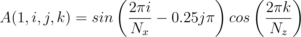
The previous section, although an important test is not particularly exciting. In this section, a more interesting visual example is presented which uses the python interface and matplotlib to plot results. A fortran and C++ example MD code specifies a test sinusoidal function in x, y and z of the form and sends this to a python CFD code which plots the results. The fortran and C++ codes are almost identical to the previous example , although this time the MD code sends to the CFD.
MD fortran send code
program MD_cpl_example
    use cpl, only : CPL_init, CPL_setup_MD, &
                    CPL_get_olap_limits, CPL_my_proc_portion, &
                    CPL_get_no_cells, CPL_send, CPL_recv, &
                    CPL_finalize
    use mpi
    implicit none

    logical :: recv_flag, send_flag, NO_ERROR
    integer :: i,j,k,ii,jj,kk,ierr
    integer :: NPx, NPy, NPz, NProcs, rank
    integer :: nprocs_realm
    integer :: CART_COMM, MD_COMM
    integer, parameter :: md_realm=2
    integer, dimension(3) :: npxyz, Ncells
    integer, dimension(6) :: portion, limits
    double precision, parameter :: pi = 3.14159265359
    double precision, dimension(3)  :: xyzL, xyz_orig
    double precision, dimension(:,:,:,:), &
         allocatable  :: send_array

    !Initialise MPI
    call MPI_Init(ierr)

    !Create MD Comm by spliting world
    call CPL_init(MD_realm, MD_COMM, ierr)

    ! Parameters of the cpu topology (cartesian grid)
    xyzL = (/10.d0, 10.d0, 10.d0/)
    xyz_orig = (/0.d0, 0.d0, 0.d0/)
    npxyz = (/ 2, 2, 1/)

    ! Create communicators and check that number of processors is consistent
    call MPI_Comm_size(MD_COMM, nprocs_realm, ierr)
    if (nprocs_realm .ne. product(npxyz)) then
        print'(4(a,i6))', "Non-coherent number of processes in MD ", nprocs_realm, &
                " no equal to ",  npxyz(1), " X ", npxyz(2), " X ", npxyz(3)
        call MPI_Abort(MPI_COMM_WORLD, 1, ierr)
    endif

    !Setup cartesian topology
    call MPI_comm_rank(MD_COMM, rank, ierr)
    call MPI_Cart_create(MD_COMM, 3, npxyz, (/1, 1, 1/), &
                         .true., CART_COMM, ierr)

    !Coupler setup
    call CPL_setup_md(CART_COMM, xyzL, xyz_orig)

    !Get detail for grid
    call CPL_get_olap_limits(limits)
    call CPL_my_proc_portion(limits, portion)
    call CPL_get_no_cells(portion, Ncells)

    ! Pack send_array with cell coordinates. Each cell in the array carries
    ! its global cell number within the overlap region.
    allocate(send_array(1, Ncells(1), Ncells(2), Ncells(3)))
    do i = 1,Ncells(1)
    do j = 1,Ncells(2)
    do k = 1,Ncells(3)
        ! -2 indices to match c++ and python indexing in portion and i,j,k
        ii = i + portion(1) - 2
        jj = j + portion(3) - 2
        kk = k + portion(5) - 2

        send_array(1,i,j,k) = sin(2.d0*pi*ii/Ncells(1)-0.25d0*jj*pi)*cos(2.d0*pi*kk/Ncells(3))
    enddo
    enddo
    enddo
    call CPL_send(send_array, limits, send_flag)

    !Release all coupler comms
    call CPL_finalize(ierr)

    !Deallocate arrays and finalise MPI
    deallocate(send_array)
    call MPI_finalize(ierr)

end program MD_cpl_example
MD C++ send code
#include "mpi.h"
#include <iostream>
#include <math.h>       /* sin */

#include "cpl.h"
#include "CPL_ndArray.h"

#define pi 3.14159265359

using namespace std;

int main() {
   MPI_Init(NULL, NULL);

   int MD_realm = 2, MD_COMM;
   CPL::init(MD_realm, MD_COMM);

   // Parameters of the cpu topology (cartesian grid)
   double xyzL[3] = {10.0, 10.0, 10.0};
   double xyz_orig[3] = {0.0, 0.0, 0.0};
   int npxyz[3] = {2, 2, 1};

   int nprocs_realm;
   MPI_Comm_size(MD_COMM, &nprocs_realm);

   // Create communicators and check that number of processors is consistent
   if (nprocs_realm != (npxyz[0] * npxyz[1] * npxyz[2])) {
      cout << "Non-coherent number of processes." << endl;
      MPI_Abort(MPI_COMM_WORLD, 1);
   }

   // Setup cartesian topology
   int rank;
   MPI_Comm_rank(MD_COMM, &rank);
   int periods[3] = {1, 1, 1};
   int CART_COMM;
   MPI_Cart_create(MD_COMM, 3, npxyz, periods, true, &CART_COMM);

   // Coupler setup
   CPL::setup_md(CART_COMM, xyzL, xyz_orig);

   // Get detail for grid
   int Ncells[3];
   int olap_limits[6], portion[6];
   CPL::get_olap_limits(olap_limits);
   CPL::my_proc_portion(olap_limits, portion);
   CPL::get_no_cells(portion, Ncells);

   // Pack send_array with cell coordinates. Each cell in the array carries
   // its global cell number within the overlap region.
   int send_shape[4] = {1, Ncells[0], Ncells[1], Ncells[2]};
   CPL::ndArray<double> send_array(4, send_shape);
   int ii, jj, kk;
   for (int i = 0; i < Ncells[0]; i++) {
       ii = i + portion[0];
       for (int j = 0; j < Ncells[1]; j++) {
           jj = j + portion[2];
           for (int k = 0; k < Ncells[2]; k++) {
               kk = k + portion[4];

               send_array(0, i, j, k) = (double) sin(2.0*pi*ii/Ncells[0]-0.25*jj*pi)*cos(2.0*pi*kk/Ncells[2]);
           }
        }
    }

   CPL::send(send_array.data(), send_array.shapeData(), olap_limits);

   // Release all coupler comms
   CPL::finalize();

   MPI_Finalize();

}
The python code requires matplotlib to be installed, which for debian based systems uses,
please see the official website for more information. The python CFD code which uses matplotlib to display the data received is as follows:
CFD python receive and plot
from mpi4py import MPI
from cplpy import CPL
import numpy as np
import matplotlib.pyplot as plt

from draw_grid import draw_grid

#initialise MPI and CPL
comm = MPI.COMM_WORLD
rank = comm.Get_rank()
COMM_size = comm.Get_size()
CPL = CPL()

# Parameters of the cpu topology (cartesian grid)
npxyz = np.array([1, 1, 1], order='F', dtype=np.int32)
NProcs = np.product(npxyz)
xyzL = np.array([10.0, 10.0, 10.0], order='F', dtype=np.float64)
xyz_orig = np.array([0.0, 0.0, 0.0], order='F', dtype=np.float64)
ncxyz = np.array([16, 6, 16], order='F', dtype=np.int32)

# Initialise coupler library
CFD_COMM = CPL.init(CPL.CFD_REALM)
nprocs_realm = CFD_COMM.Get_size()

if (nprocs_realm != NProcs):
    print(("Non-coherent number of processes in CFD ", nprocs_realm,
            " no equal to ",  npxyz[0], " X ", npxyz[1], " X ", npxyz[2]))
    MPI.Abort(errorcode=1)

#Setup coupled simulation
cart_comm = CFD_COMM.Create_cart([npxyz[0], npxyz[1], npxyz[2]])
CPL.setup_cfd(cart_comm, xyzL, xyz_orig, ncxyz)

# recv data to plot
olap_limits = CPL.get_olap_limits()
portion = CPL.my_proc_portion(olap_limits)
[ncxl, ncyl, nczl] = CPL.get_no_cells(portion)
recv_array = np.zeros((1, ncxl, ncyl, nczl), order='F', dtype=np.float64)
recv_array, ierr = CPL.recv(recv_array, olap_limits)

#Plot output
fig, ax = plt.subplots(2,1)

#Plot x component on grid
for j in range(CPL.get("jcmin_olap"),CPL.get("jcmax_olap")+1):
    ax[0].plot((recv_array[0,:,j,0]+1.+2*j), 's-')
ax[0].set_xlabel('$x$')
ax[0].set_ylabel('$y$')

#Plot xz of bottom cell
ax[1].pcolormesh(recv_array[0,:,0,:])
ax[1].set_xlabel('$x$')
ax[1].set_ylabel('$z$')
plt.show()

CPL.finalize()
MPI.Finalize()


# === Plot both grids ===
dx = CPL.get("xl_cfd")/float(CPL.get("ncx"))
dy = CPL.get("yl_cfd")/float(CPL.get("ncy"))
dz = CPL.get("zl_cfd")/float(CPL.get("ncz"))
ioverlap = (CPL.get("icmax_olap")-CPL.get("icmin_olap")+1)
joverlap = (CPL.get("jcmax_olap")-CPL.get("jcmin_olap")+1)
koverlap = (CPL.get("kcmax_olap")-CPL.get("kcmin_olap")+1)
xoverlap = ioverlap*dx
yoverlap = joverlap*dy
zoverlap = koverlap*dz

#Plot CFD and coupler Grid
draw_grid(ax[0],
          nx=CPL.get("ncx"),
          ny=CPL.get("ncy"),
          nz=CPL.get("ncz"),
          px=CPL.get("npx_cfd"),
          py=CPL.get("npy_cfd"),
          pz=CPL.get("npz_cfd"),
          xmin=xyz_orig[0],
          ymin=xyz_orig[1],
          zmin=xyz_orig[2],
          xmax=(CPL.get("icmax_olap")+1)*dx,
          ymax=CPL.get("yl_cfd"),
          zmax=(CPL.get("kcmax_olap")+1)*dz,
          lc = 'r',
          label='CFD')

#Plot MD domain
draw_grid(ax[0], nx=1, ny=1, nz=1,
          px=CPL.get("npx_md"),
          py=CPL.get("npy_md"),
          pz=CPL.get("npz_md"),
          xmin=CPL.get("icmin_olap")*dx,
          ymin=-CPL.get("yl_md")+yoverlap,
          zmin=-CPL.get("kcmin_olap")*dz,
          xmax=(CPL.get("icmax_olap")+1)*dx,
          ymax=yoverlap,
          zmax=(CPL.get("kcmax_olap")+1)*dz,
          label='MD')

#Plot some random molecules
#ax[0].plot(np.random.random(100)*(CPL.get("xl_md")),
#           np.random.random(100)*(CPL.get("yl_md"))-CPL.get("yl_md")+yoverlap,
#           'ob',alpha=0.5)

#print(CPL.get("icmin_olap"),CPL.get("icmax_olap")+1,float(CPL.get("ncx")),CPL.get("zl_cfd"),dz)
#for i in range(CPL.get("icmin_olap"),CPL.get("icmax_olap")+1):
#    for j in range(CPL.get("jcmin_olap"),CPL.get("jcmax_olap")+1):
#        #for k in range(CPL.get("kcmin_olap"),CPL.get("kcmax_olap")):

#        ax[0].text(i*dx,j*dy,str(i)+","+str(j))

#Plot x component on grid
x = np.linspace(.5*dx,xoverlap-.5*dx,ioverlap)
z = np.linspace(.5*dz,zoverlap-.5*dz,koverlap)
for j in range(joverlap):
    ax[0].plot(x, 0.5*dy*(recv_array[0,:,j,0]+1.+2*j), 's-')
ax[0].set_xlabel('$x$')
ax[0].set_ylabel('$y$')

#Plot xz of bottom cell
X,Z = np.meshgrid(z,x)
ax[1].pcolormesh(X,Z,recv_array[0,:,0,:])
ax[1].set_xlabel('$x$')
ax[1].set_ylabel('$z$')
plt.show()

CPL.finalize()
MPI.Finalize()
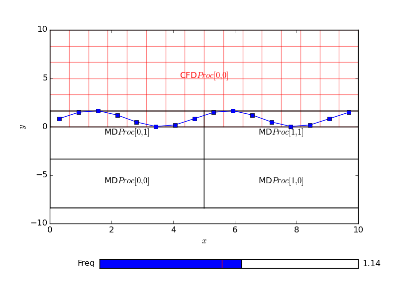
Setting the cells to be a combination of sines and cosines for every cell in the domain, here set to be 16 by 16 in x and z. The CFD code has 6 cell with an overlap size specified to be 4 cells,
This plots a figure of the form,
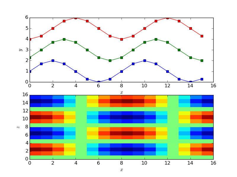
The grid is set to a function of x, y and z based on cell numbers. The above plot shows the x and y dependence of the functions on the top figure and the x z dependence on the bottom layer. In order to understand this in the context of the coupler grid, a python function can be used to add a grid to the plot,
Python Grid plotting function
import numpy as np
import matplotlib.pyplot as plt

def draw_lines(ax, x, y, lc, lw=1., XKCD_plots=False):

    if XKCD_plots:
        from XKCD_plot_generator import xkcd_line

    for n in range(x.size):
        if XKCD_plots:
            xp, yp = xkcd_line([x[n], x[n]],  [y[0], y[-1]])
        else:
            xp, yp = [x[n], x[n]],  [y[0], y[-1]]
        ax.plot(xp, yp, '-'+lc,lw=lw,alpha=0.5)
    for n in range(y.size):
        if XKCD_plots:
            xp, yp = xkcd_line([x[0], x[-1]], [y[n], y[n]])
        else:
            xp, yp = [x[0], x[-1]], [y[n], y[n]]
        ax.plot(xp, yp, '-'+lc,lw=lw,alpha=0.5)


def draw_grid(ax, nx, ny, nz,
              px=1, py=1, pz=1,
              xmin=0.,ymin=0.,zmin=0.,
              xmax=1.,ymax=1.,zmax=1.,
              ind=0., fc='r', lc='k',
              offset=0., label="",
              nodes=False,
              XKCD_plots=False, **kwargs):

    ymin += offset
    ymax += offset

    x = np.linspace(xmin, xmax, nx+1)
    y = np.linspace(ymin, ymax, ny+1)
    z = np.linspace(zmin, zmax, nz+1)
    if nodes:
        X,Y,Z = np.meshgrid(x,y,z)
        self.ax.plot(X[:,:,ind],Y[:,:,ind],'s'+fc,alpha=0.5)

    draw_lines(ax, x, y, lc=lc,XKCD_plots=XKCD_plots)

    xp = np.linspace(xmin, xmax, px+1)
    yp = np.linspace(ymin, ymax, py+1)
    zp = np.linspace(zmin, zmax, pz+1)
    if nodes:
        X,Y,Z = np.meshgrid(xp,yp,zp)
        ax.plot(X[:,:,ind],Y[:,:,ind],'s'+fc,alpha=0.5)

    draw_lines(ax, xp, yp, lc='k',lw=2,XKCD_plots=XKCD_plots)

    #Annotate the processors
    dxp = np.mean(np.diff(xp))
    dyp = np.mean(np.diff(yp))
    #Make some effort to ensure the text fits on a normal screen
    if px > 8 or py > 8:
        fontsize = 8
    else:
        fontsize = 12
    for i,px in enumerate(xp[1:]):
        for j,py in enumerate(yp[1:]):
            ax.text(px-.5*dxp,py-.5*dyp,
                    label+"$ Proc [" + str(i) + "," + str(j) + "]$",
                    horizontalalignment="center",color=lc,
                    fontsize=fontsize)
There are no changes needed to the sending code. The python code to use this in the plot introduced the cpl_get function in order to obtain the grid properties. All details of the coupled configuration are stored locally on every processor so no communication is required for a call to CPL_get. The code receive data and plots over the grid resulting the following,
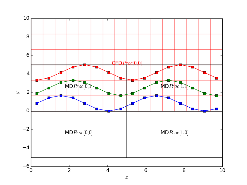
Notice that the MD code is running on four processor, highlighted on the grid plot and the sine function is clearly continuous and correct over the processor boundaries. A single CFD processor receives and plots the data for simplicity here. The CPL could be used in this manner on an MD or CFD simulation running on thousands of processors and the CPL library linked only to display current values. By linking to a particular location, a slice or plot along an axis could be used without requiring global communications. In this way, the current state of the simulation can be checked while maintaining the scaling of the codes. This is a very important function to use when developing coupled simulation. As typically you will be linking two highly complex and non-linear codes, they MUST be verified individually before attempting to link. Using the python interface with plotting, the two codes can be visualised, unit-tested and verified individually. The simple plotting interface can then be simply swapped out for the other code. Both for debugging and controlling simulation, CPL library can be used to not only display the current state of the simulation, but also to control it by specifying a boundary condition. In the next section, the plotting code sends back a user changeable value to interactively develop a coupled simulation.
Demo: Interactive GUI using CPL library
This allows an interactive code to adjust the various values, usign a send and receive. The python code to do this uses matplotlib widgets and is as follows,
Interactive python code
import numpy as np
import matplotlib.pyplot as plt
from matplotlib.widgets import Slider
from mpi4py import MPI

from cplpy import CPL
from draw_grid import draw_grid

#initialise MPI and CPL
comm = MPI.COMM_WORLD
CPL = CPL()
CFD_COMM = CPL.init(CPL.CFD_REALM)
nprocs_realm = CFD_COMM.Get_size()

# Parameters of the cpu topology (cartesian grid)
npxyz = np.array([1, 1, 1], order='F', dtype=np.int32)
NProcs = np.product(npxyz)
xyzL = np.array([10.0, 10.0, 10.0], order='F', dtype=np.float64)
xyz_orig = np.array([0.0, 0.0, 0.0], order='F', dtype=np.float64)
ncxyz = np.array([16, 6, 16], order='F', dtype=np.int32)

if (nprocs_realm != NProcs):
    print(("Non-coherent number of processes in CFD ", nprocs_realm,
            " no equal to ",  npxyz[0], " X ", npxyz[1], " X ", npxyz[2]))
    MPI.Abort(errorcode=1)

#Setup coupled simulation
cart_comm = CFD_COMM.Create_cart([npxyz[0], npxyz[1], npxyz[2]])
CPL.setup_cfd(cart_comm, xyzL, xyz_orig, ncxyz)

#Plot output
fig, ax = plt.subplots(1,1)
plt.subplots_adjust(bottom=0.25)
axslider = plt.axes([0.25, 0.1, 0.65, 0.03])
freq = 1.
sfreq = Slider(axslider, 'Freq', 0.1, 2.0, valinit=freq)
def update(val):
    freq = sfreq.val
    global freq
    print(("CHANGED", freq))
sfreq.on_changed(update)

plt.ion()
plt.show()

# === Plot both grids ===
dx = CPL.get("xl_cfd")/float(CPL.get("ncx"))
dy = CPL.get("yl_cfd")/float(CPL.get("ncy"))
dz = CPL.get("zl_cfd")/float(CPL.get("ncz"))
ioverlap = (CPL.get("icmax_olap")-CPL.get("icmin_olap")+1)
joverlap = (CPL.get("jcmax_olap")-CPL.get("jcmin_olap")+1)
koverlap = (CPL.get("kcmax_olap")-CPL.get("kcmin_olap")+1)
xoverlap = ioverlap*dx
yoverlap = joverlap*dy
zoverlap = koverlap*dz

for time in range(100000):

    # recv data to plot
    olap_limits = CPL.get_olap_limits()
    portion = CPL.my_proc_portion(olap_limits)
    [ncxl, ncyl, nczl] = CPL.get_no_cells(portion)
    recv_array = np.zeros((1, ncxl, ncyl, nczl), order='F', dtype=np.float64)
    recv_array, ierr = CPL.recv(recv_array, olap_limits)

    #Plot CFD and coupler Grid
    draw_grid(ax,
              nx=CPL.get("ncx"),
              ny=CPL.get("ncy"),
              nz=CPL.get("ncz"),
              px=CPL.get("npx_cfd"),
              py=CPL.get("npy_cfd"),
              pz=CPL.get("npz_cfd"),
              xmin=CPL.get("x_orig_cfd"),
              ymin=CPL.get("y_orig_cfd"),
              zmin=CPL.get("z_orig_cfd"),
              xmax=(CPL.get("icmax_olap")+1)*dx,
              ymax=CPL.get("yl_cfd"),
              zmax=(CPL.get("kcmax_olap")+1)*dz,
              lc = 'r',
              label='CFD')

    #Plot MD domain
    draw_grid(ax, nx=1, ny=1, nz=1,
              px=CPL.get("npx_md"),
              py=CPL.get("npy_md"),
              pz=CPL.get("npz_md"),
              xmin=CPL.get("x_orig_md"),
              ymin=-CPL.get("yl_md")+yoverlap,
              zmin=CPL.get("z_orig_md"),
              xmax=(CPL.get("icmax_olap")+1)*dx,
              ymax=yoverlap,
              zmax=(CPL.get("kcmax_olap")+1)*dz,
              label='MD')

    #Plot x component on grid
    x = np.linspace(CPL.get("x_orig_cfd")+.5*dx,xoverlap-.5*dx,ioverlap)
    z = np.linspace(CPL.get("z_orig_cfd")+.5*dz,zoverlap-.5*dz,koverlap)
    for j in range(joverlap):
        ax.plot(x, 0.5*dy*(recv_array[0,:,j,0]+1.+2*j), 's-')
    ax.set_xlabel('$x$')
    ax.set_ylabel('$y$')

    print((time, freq))
    plt.pause(0.1)
    ax.cla()

    # send data to update
    olap_limits = CPL.get_olap_limits()
    portion = CPL.my_proc_portion(olap_limits)
    [ncxl, ncyl, nczl] = CPL.get_no_cells(portion)
    send_array = freq*np.ones((1, ncxl, ncyl, nczl), order='F', dtype=np.float64)
    CPL.send(send_array, olap_limits)

CPL.finalize()
MPI.Finalize()
The previous MD code needs to be adapted to receive data from the
CFD code, as well as evolve in time to reflect the potentially changing
boundary.
Interactive fortran code
program MD_cpl_example
    use cpl, only : CPL_init, CPL_setup_MD, &
                    CPL_get_olap_limits, CPL_my_proc_portion, &
                    CPL_get_no_cells, CPL_send, CPL_recv, &
                    CPL_finalize
    use mpi
    implicit none

    logical :: recv_flag, send_flag, NO_ERROR
    integer :: i,j,k,ii,jj,kk,ierr
    integer :: NPx, NPy, NPz, NProcs, rank
    integer :: nprocs_realm, time
    integer :: CART_COMM, MD_COMM
    integer, parameter :: md_realm=2
    integer, dimension(3) :: npxyz, Ncells
    integer, dimension(6) :: portion, limits
    double precision, parameter :: pi = 3.14159265359
    double precision, dimension(3)  :: xyzL, xyz_orig
    double precision, dimension(:,:,:,:), &
         allocatable  :: send_array, recv_array

    !Initialise MPI
    call MPI_Init(ierr)

    !Create MD Comm by spliting world
    call CPL_init(MD_realm, MD_COMM, ierr)

    ! Parameters of the cpu topology (cartesian grid)
    xyzL = (/10.d0, 10.d0, 10.d0/)
    xyz_orig = (/0.d0, 0.d0, 0.d0/)
    npxyz = (/ 2, 2, 1/)

    ! Create communicators and check that number of processors is consistent
    call MPI_Comm_size(MD_COMM, nprocs_realm, ierr)
    if (nprocs_realm .ne. product(npxyz)) then
        print'(4(a,i6))', "Non-coherent number of processes in MD ", nprocs_realm, &
                " no equal to ",  npxyz(1), " X ", npxyz(2), " X ", npxyz(3)
        call MPI_Abort(MPI_COMM_WORLD, 1, ierr)
    endif

    !Setup cartesian topology
    call MPI_comm_rank(MD_COMM, rank, ierr)
    call MPI_Cart_create(MD_COMM, 3, npxyz, (/1, 1, 1/), &
                         .true., CART_COMM, ierr)

    !Coupler setup
    call CPL_setup_md(CART_COMM, xyzL, xyz_orig)

    !Get detail for grid
    call CPL_get_olap_limits(limits)
    call CPL_my_proc_portion(limits, portion)
    call CPL_get_no_cells(portion, Ncells)

    allocate(send_array(1, Ncells(1), Ncells(2), Ncells(3)))
    allocate(recv_array(1, Ncells(1), Ncells(2), Ncells(3)))
    send_array = 0.d0; recv_array = 1.d0
    do time = 1,10000

        ! Pack send_array with cell coordinates. Each cell in the array carries
        ! its global cell number within the overlap region.
        do i = 1,Ncells(1)
        do j = 1,Ncells(2)
        do k = 1,Ncells(3)
            ! -2 indices to match c++ and python indexing in portion and i,j,k
            ii = i + portion(1) - 2
            jj = j + portion(3) - 2
            kk = k + portion(5) - 2

            send_array(1,i,j,k) =sin(recv_array(1,i,j,k)*2.d0*pi*ii/Ncells(1) &
                                 -0.25d0*jj*pi) *cos(2.d0*pi*kk/Ncells(3))

        enddo
        enddo
        enddo
        call CPL_send(send_array, limits, send_flag)

        !Recv array of updated sin coefficients data
        call CPL_recv(recv_array, limits, recv_flag)

    enddo

    !Release all coupler comms
    call CPL_finalize(ierr)

    !Deallocate arrays and finalise MPI
    deallocate(send_array)
    call MPI_finalize(ierr)

end program MD_cpl_example
Interactive cpp code
#include "cpl.h"
#include "mpi.h"
#include <iostream>
#include <math.h>       /* sin */

#define pi 3.14159265359

#include "CPL_ndArray.h"

using namespace std;

int main() {
   MPI_Init(NULL, NULL);

   int MD_realm = 2, MD_COMM;
   CPL::init(MD_realm, MD_COMM);

   // Parameters of the cpu topology (cartesian grid)
   double xyzL[3] = {10.0, 10.0, 10.0};
   double xyz_orig[3] = {0.0, 0.0, 0.0};
   int npxyz[3] = {2, 2, 1};

   int nprocs_realm;
   MPI_Comm_size(MD_COMM, &nprocs_realm);

   // Create communicators and check that number of processors is consistent
   if (nprocs_realm != (npxyz[0] * npxyz[1] * npxyz[2])) {
      cout << "Non-coherent number of processes." << endl;
      MPI_Abort(MPI_COMM_WORLD, 1);
   }

   // Setup cartesian topology
   int rank;
   MPI_Comm_rank(MD_COMM, &rank);
   int periods[3] = {1, 1, 1};
   int CART_COMM;
   MPI_Cart_create(MD_COMM, 3, npxyz, periods, true, &CART_COMM);

   // Coupler setup
   CPL::setup_md(CART_COMM, xyzL, xyz_orig);

   // Get detail for grid
   int Ncells[3];
   int olap_limits[6], portion[6];
   CPL::get_olap_limits(olap_limits);
   CPL::my_proc_portion(olap_limits, portion);
   CPL::get_no_cells(portion, Ncells);

   // Pack send_array with cell coordinates. Each cell in the array carries
   // its global cell number within the overlap region.
   int send_shape[4] = {1, Ncells[0], Ncells[1], Ncells[2]};
   int recv_shape[4] = {1, Ncells[0], Ncells[1], Ncells[2]};
   CPL::ndArray<double> send_array(4, send_shape);
   CPL::ndArray<double> recv_array(4, recv_shape);
   int ii, jj, kk;

   for (int time = 0; time < 100000; time++){
       for (int i = 0; i < Ncells[0]; i++) {
           ii = i + portion[0];
           for (int j = 0; j < Ncells[1]; j++) {
               jj = j + portion[2];
               for (int k = 0; k < Ncells[2]; k++) {
                   kk = k + portion[4];

                   send_array(0, i, j, k) = (double) sin(recv_array(0, i, j, k)*2.0*pi*ii/Ncells[0]
                                                         -0.25*jj*pi)
                                                    *cos(2.0*pi*kk/Ncells[2]);
               }
            }
        }

       //Send data
       CPL::send(send_array.data(), send_array.shapeData(), olap_limits);

       //Recv array of coefficients
       CPL::recv(recv_array.data(), recv_array.shapeData(), olap_limits);

   }

   // Release all coupler comms
   CPL::finalize();

   MPI_Finalize();

}
Minimal CFD and MD code with coupling
Bringing the previous examples of topological setup and data exchange, along with a minimal CFD solver for the 2D unsteady diffusive equation,
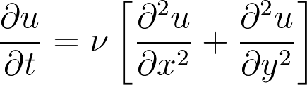
This equation is simulated using a simple finite difference method with a forward Euler for time discretisation and central difference in space. The code is written in an object oriented manner, so a CFD object can be created, containing all field information and allowing specification of boundary conditions, time evolution and plotting:
CFD code
import numpy as np
import matplotlib.pyplot as plt

from draw_grid import draw_grid

class CFD:
    """
        Solve the diffusion equation
        du/dt = (rho/gamma) * d2u/dx2
    """
    def __init__(self, dt, nu = 1.,
                 xsize = 10, ysize = 10,
                 xmin = 0., xmax = 1.,
                 ymin = 0., ymax = 1.,
                 fig=None):

        #Define coefficients
        self.nu = nu
        self.xsize = xsize
        self.ysize = ysize
        self.xmin = xmin
        self.xmax = xmax
        self.ymin = ymin
        self.ymax = ymax
        self.dt = dt

        #Define arrays
        self.x = np.linspace(xmin,xmax,xsize)
        self.dx = np.mean(np.diff(self.x))
        self.y = np.linspace(ymin,ymax,ysize)
        self.dy = np.mean(np.diff(self.y))

        #For plotting
        self.X,self.Y = np.meshgrid(self.x,self.y)

        #Check CFL stability conditions
        self.CFL =  (1./(2.*nu))*(self.dx*self.dy)**2/(self.dx**2+self.dy**2)
        if self.dt > self.CFL:
            print(("Stability conditions violated, CFL=", self.CFL ,
                  "> dt=", self.dt," adjust dt, nu or grid spacing"))
            quit()
        else:
            print(("Timestep dt = ", self.dt, " CFL number= ", self.CFL))

        #initial condition
        self.u0 = np.zeros([xsize,ysize])

        #Setup first times
        self.u = np.copy(self.u0)
        self.u_mdt =  np.copy(self.u0)
        self.u_m2dt =  np.copy(self.u0)
        self.first_time = True

        #Setup figure
        if fig ==  None:
            self.fig, self.ax = plt.subplots(1,1)
            plt.ion()
            plt.show()
        else:
            self.fig = fig
            self.ax = fig.axes

    def set_bc(self, topwall=1., bottomwall=0.):
        #Periodic boundaries
        self.u[-1,1:-1] = self.u[1,1:-1]; self.u[0,1:-1] = self.u[-2,1:-1]
        #Enforce boundary conditions
        self.u[:,0] = bottomwall; self.u[:,-1] = topwall


    def update_time(self):
        # Save previous value
        self.u_m2dt = np.copy(self.u_mdt)
        self.u_mdt = np.copy(self.u)

        #Solve for new u
        for i in range(1,self.x.size-1):
            for j in range(1,self.y.size-1):
                #Diffusion equation, forward Euler
                self.u[i,j] = self.u_mdt[i,j] + self.nu*self.dt*(
                                (self.u_mdt[i+1,j]-2.*self.u_mdt[i,j]+self.u_mdt[i-1,j])/self.dx**2
                               +(self.u_mdt[i,j+1]-2.*self.u_mdt[i,j]+self.u_mdt[i,j-1])/self.dy**2)

    #Plot graph
    def plot(self, ax=None):
        if ax == None:
            ax=self.ax

        if type(ax) is list:
            ax  = ax[0]

        sm = ax.imshow(self.u.T, aspect='auto', origin='lower',
                       extent=[self.xmin, self.xmax,
                               self.ymin, self.ymax],
                       interpolation="none", vmin=-1., vmax=1.,
                       alpha=0.5, cmap=plt.cm.RdYlBu_r)

#        sm = ax.pcolormesh(self.X,self.Y,self.u.T,vmin=-1.,vmax=1.,alpha=0.5,
#                          cmap=plt.cm.RdYlBu_r)
        draw_grid(ax, nx=self.x.size,ny=self.y.size, nz=1,
                      xmin=self.xmin,xmax=self.xmax,
                      ymin=self.ymin,ymax=self.ymax)

        #Plot velocity profile offset to the left
        axisloc = self.xmax+1.

        ax.arrow(axisloc, 0., self.ymin, self.ymax,  width=0.0015, color="k",
                 clip_on=False, head_width=0.12, head_length=0.12)
        mid = .5*(self.ymin+self.ymax)
        ax.arrow(axisloc-1., mid, 2.0, 0., width=0.0015, color="k",
                 clip_on=False, head_width=0.12, head_length=0.12)
        yp = np.linspace(self.ymin+.5*self.dy, self.ymax - 0.5*self.dy, self.y.size)
        ax.plot(np.mean(self.u,0)+axisloc,yp,'g-x')
        #ax.set_xlim((0.,2.))

        if self.first_time:
            plt.colorbar(sm)
            self.first_time=False

        plt.pause(0.001)
        ax.cla()

if __name__ == "__main__":

    t0 = 0; tf = 30.; Nsteps = 10000
    time = np.linspace(t0, tf, Nsteps)
    dt = np.mean(np.diff(time))
    uwall = 1.
    ncx = 8; ncy = 8
    xl_cfd = 1.; yl_cfd = 1.

    fig, ax = plt.subplots(1,1)

    cfd = CFD(nu=0.575, dt=dt, fig=fig,
              xsize = ncx, ysize = ncy+2,
              xmin = 0., xmax = xl_cfd,
              ymin = 0., ymax = yl_cfd)

    for n,t in enumerate(time):

        print(("CFD time = ", n,t))

        #===============================================
        # Call to CPL-LIBRARY goes here to
        # recieve u_MD to set bottom boundary
        #===============================================
        #umd = cpl.recv(u)
        #bottomwall = np.mean(umd)

        #Update CFD
        cfd.set_bc(topwall=uwall, bottomwall=0.)
        cfd.update_time()
        cfd.plot()

        #===============================================
        # Call to CPL-LIBRARY goes here to
        # send u_CFD in constraint region
        #===============================================
        #ucnst = cfd.u[:,7]
The minimal MD code solves Newton's law for the N body problem. This is extremely slow in python so only a very small number of molecules are used. A simply cell list is also included to speed up the simulation and time is advanced using a Verlet algorithm. A number of non-equilibrium molecular dynamics and coupling specific features are required, including fixed wall molecules, a specular wall at the domain top, constraint force and averaging to get a velocity field. The MD code is also written in an object oriented manner with functions for force calculation, time evolution and plotting along with more exotic velocity averaging, constraint forces and specular walls.
MD code
import numpy as np
import matplotlib.pyplot as plt
from draw_grid import draw_grid
class MD:
def __init__(self,
initialnunits = [3,8],
density = 0.8,
nd = 2,
rcutoff = 2.**(1./6.),
dt = 0.005,
Tset = 1.3, #After equilbirum approx temp of 1
forcecalc = "allpairs",
wallwidth = [0.,0.],
wallslide = [0.,0.],
newfig=None):
self.initialnunits = initialnunits
self.density = density
self.nd = nd
self.rcutoff = rcutoff
self.dt = dt
self.forcecalc = forcecalc
self.wallwidth = np.array(wallwidth)
self.wallslide = np.array(wallslide)
self.rcutoff2 = rcutoff**2
self.first_time=True
self.tstep = 0
self.time = 0.
self.periodic = [True, True]
self.spec_wall = [False, False]
#Setup Initial crystal
self.domain = np.zeros(2)
self.volume=1. #Set domain size to unity for loop below
for ixyz in range(nd):
self.domain[ixyz] = (initialnunits[ixyz]/((density/4.0)**(1.0/nd)))
self.volume = self.volume*self.domain[ixyz] #Volume based on size of domain
self.halfdomain = 0.5*self.domain
#Allocate arrays
self.N = 4*initialnunits[0]*initialnunits[1]
self.tag = np.zeros(self.N, dtype=int)
self.r = np.zeros((self.N,2))
self.v = np.zeros((self.N,2))
self.a = np.zeros((self.N,2))
self.v = Tset*np.random.randn(self.v.shape[0], self.v.shape[1])
vsum = np.sum(self.v,0)/self.N
for i in range(self.N):
self.v[i,:] -= vsum
#Setup velocity averaging
self.veluptodate = 0
self.xbin = 8; self.ybin = 8
self.dx = self.domain[0]/self.xbin
self.dy = self.domain[1]/self.ybin
self.xb = np.linspace(-self.halfdomain[0],
self.halfdomain[0], self.xbin)
self.yb = np.linspace(-self.halfdomain[1],
self.halfdomain[1], self.ybin)
self.Xb, self.Yb = np.meshgrid(self.xb, self.yb)
self.mbin = np.zeros([self.xbin, self.ybin])
self.velbin = np.zeros([2, self.xbin, self.ybin])
self.setup_crystal()
self.setup_walls(wallwidth)
if newfig == None:
self.fig, self.ax = plt.subplots(1,1)
plt.ion()
plt.show()
#Molecules per unit FCC structure (3D)
def setup_crystal(self):
initialunitsize = self.domain / self.initialnunits
n = 0 #Initialise global N counter n
c = np.zeros(2); rc = np.zeros(2)
for nx in range(1,self.initialnunits[0]+1):
c[0] = (nx - 0.750)*initialunitsize[0]
for ny in range(1,self.initialnunits[1]+1):
c[1] = (ny - 0.750)*initialunitsize[1]
for j in range(4): #4 Molecules per cell
rc[:] = c[:]
if j is 1:
rc[0] = c[0] + 0.5*initialunitsize[0]
elif j is 2:
rc[1] = c[1] + 0.5*initialunitsize[1]
elif j is 3:
rc[0] = c[0] + 0.5*initialunitsize[0]
rc[1] = c[1] + 0.5*initialunitsize[1]
#Correct to local coordinates
self.r[n,0] = rc[0]-self.halfdomain[0]
self.r[n,1] = rc[1]-self.halfdomain[1]
n += 1 #Move to next particle
def setup_walls(self, wallwidth):
for i in range(self.N):
if (self.r[i,1]+self.halfdomain[1] < wallwidth[0]):
self.tag[i] = 1
elif (self.r[i,1]+self.halfdomain[1] > self.domain[1]-wallwidth[1]):
self.tag[i] = 1
else:
self.tag[i] = 0
if any(self.wallwidth > 0.):
self.periodic[1] = False
self.spec_wall[1] = True
def LJ_accij(self,rij2):
invrij2 = 1./rij2
return 48.*(invrij2**7-.5*invrij2**4)
def get_bin(self, r, binsize):
ib = [int((r[ixyz]+0.5*self.domain[ixyz])
/binsize[ixyz]) for ixyz in range(self.nd)]
return ib
def get_velfield(self, bins, freq=25, plusdt=False, getmbin=False):
#Update velocity if timestep dictates
if ((self.tstep%freq == 0)
and (self.tstep != self.veluptodate)):
mbin = np.zeros([bins[0], bins[1]])
velbin = np.zeros([2, bins[0], bins[1]])
binsize = self.domain/bins
#Loop over all molecules in r
for i in range(self.r.shape[0]):
ib = self.get_bin(self.r[i,:], binsize)
mbin[ib[0], ib[1]] += 1
if plusdt:
vi = self.v[i,:] + self.dt*self.a[i,:]
else:
vi = self.v[i,:]
velbin[:, ib[0], ib[1]] += vi
self.mbin = mbin
self.velbin = velbin
self.veluptodate = self.tstep
else:
mbin = self.mbin
velbin = self.velbin
u = np.divide(velbin,mbin)
u[np.isnan(u)] = 0.0
if getmbin:
return u, mbin
else:
return u
def force(self, showarrows=False, ax=None):
if ax == None:
ax=self.ax
#Force calculation
self.a = np.zeros((self.N,2))
if self.forcecalc is "allpairs":
for i in range(self.N):
for j in range(i+1,self.N):
ri = self.r[i,:]; rj = self.r[j,:]
rij = ri - rj
#Nearest neighbour
for ixyz in range(self.nd):
if self.periodic[ixyz]:
if (np.abs(rij[ixyz]) > self.halfdomain[ixyz]):
rij[ixyz] -= np.copysign(self.domain[ixyz],rij[ixyz])
#Get forces
rij2 = np.dot(rij,rij)
if rij2 < self.rcutoff2:
fij = self.LJ_accij(rij2)*rij
self.a[i,:] += fij
self.a[j,:] -= fij
if showarrows:
ax.quiver(self.r[i,0],self.r[i,1],
rij[0], rij[1],color='red',width=0.002)
ax.quiver(self.r[j,0],self.r[j,1],
-rij[0],-rij[1],color='red',width=0.002)
elif "celllist":
#Build celllist
self.cells = [int(self.domain[i]/(self.rcutoff)) for i in range(self.nd)]
self.cell = np.zeros(self.cells, dtype=object)
for icell in range(self.cells[0]):
for jcell in range(self.cells[1]):
self.cell[icell,jcell] = []
cellsize = self.domain/cells
for i in range(self.N):
ib = self.get_bin(r[i,:], cellsize)
self.cell[ib[0],ib[1]].append(i)
#For each cell, check molecule i
for icell in range(self.cells[0]):
for jcell in range(self.cells[1]):
for i in cell[icell,jcell]:
ri = self.r[i,:]
#Check i against all molecules in adjacent cells
for aicell in [icell-1,icell,(icell+1)%cells[0]]:
for ajcell in [jcell-1,jcell,(jcell+1)%cells[1]]:
for j in cell[aicell,ajcell]:
rj = self.r[j,:]
rij = ri - rj
#Nearest neighbour
for ixyz in range(nd):
if self.periodic[ixyz]:
if (np.abs(rij[ixyz]) > self.halfdomain[ixyz]):
rij[ixyz] -= np.copysign(self.domain[ixyz],rij[ixyz])
#Get forces
rij2 = np.dot(rij,rij)
if rij2 < self.rcutoff2 and rij2 > 1e-8:
fij = self.LJ_accij(rij2)*rij
self.a[i,:] += fij
if showarrows:
ax.quiver(self.r[i,0],self.r[i,1],
-rij[0],-rij[1],color='red',width=0.002)
def verlet(self):
#Verlet time advance
for i in range(self.N):
if self.tag[i] == 0:
self.v[i,:] += self.dt*self.a[i,:]
self.r[i,:] += self.dt*self.v[i,:]
else:
#Fixed molecule, add sliding
self.v[i,:] = self.wallslide[:]
self.r[i,:] += self.dt*self.wallslide[:]
#Peridic boundary and specular wall
for ixyz in range(self.nd):
if self.r[i,ixyz] > self.halfdomain[ixyz]:
if self.spec_wall[ixyz]:
overshoot = self.r[i,ixyz]-self.halfdomain[ixyz]
self.r[i,ixyz] -= 2.*overshoot
self.v[i,ixyz] = -self.v[i,ixyz]
else:
self.r[i,ixyz] -= self.domain[ixyz]
elif self.r[i,ixyz] < -self.halfdomain[ixyz]:
if self.spec_wall[ixyz]:
overshoot = -self.halfdomain[ixyz]-self.r[i,ixyz]
self.r[i,ixyz] += 2.*overshoot
self.v[i,ixyz] = -self.v[i,ixyz]
else:
self.r[i,ixyz] += self.domain[ixyz]
#Increment current time step
self.tstep += 1
self.time = self.tstep*self.dt
def constraint_force(self, u_CFD, constraint_cell, alpha=0.1):
#Get the MD velocity field
binsize_CFD = self.domain/u_CFD.shape[1:2]
binsize_MD = self.domain/[self.xbin, self.ybin]
assert binsize_CFD[0] == binsize_MD[0]
assert binsize_CFD[1] == binsize_MD[1]
u_MD, mbin = self.get_velfield([self.xbin,self.ybin], getmbin=True)
#Extract CFD value
F = np.zeros(2)
ucheck = np.zeros([2,self.xbin])
hd = self.halfdomain
for i in range(self.N):
ib = self.get_bin(self.r[i,:], binsize_MD)
#Ensure within domain
if ib[0] > u_MD.shape[1]:
ib[0] = u_MD.shape[1]
if ib[1] > u_MD.shape[2]:
ib[1] = u_MD.shape[2]
#only apply to constrained cell
if ib[1] == constraint_cell:
F[:] = alpha*(u_CFD[:,ib[0],0] - u_MD[:,ib[0],ib[1]])
if (mbin[ib[0],ib[1]] != 0):
self.a[i,:] += F[:]/float(mbin[ib[0],ib[1]])
else:
pass
self.ax.quiver((ib[0]+.5)*self.dx-hd[0],
(ib[1]+.5)*self.dy-hd[1],F[0],F[1],
color='red',angles='xy',scale_units='xy',scale=1)
def CV_constraint_force(self, u_CFD, constraint_cell):
#Get the MD velocity field
binsize_CFD = self.domain/u_CFD.shape[1:2]
binsize_MD = self.domain/[self.xbin, self.ybin]
assert binsize_CFD[0] == binsize_MD[0]
assert binsize_CFD[1] == binsize_MD[1]
u_MD = self.get_velfield([self.xbin,self.ybin], freq=1)
#Apply force value
F = np.zeros(2)
du_MDdt = np.zeros(2)
du_CFDdt = np.zeros(2)
hd = self.halfdomain
for i in range(self.N):
ib = self.get_bin(r[i,:], binsize_MD)
#Ensure within domain
if ib[0] > u_MD.shape[1]:
ib[0] = u_MD.shape[1]
if ib[1] > u_MD.shape[2]:
ib[1] = u_MD.shape[2]
#only apply to constrained cell
if ib[1] == constraint_cell:
du_MDdt[:] = (u_MD[:,ib[0],ib[1]]
- self.u_MD[:,ib[0],ib[1]])
du_CFDdt[:] = (u_CFD[:,ib[0],ib[1]]
- self.u_CFD[:,ib[0],ib[1]])
if (mbin[ib[0],ib[1]] != 0):
F[:] = ( (du_MDdt - du_CFDdt)
/(float(mbin[ib[0],ib[1]])*self.dt))
else:
F[:] = 0.
self.u_MD = u_MD
self.u_CFD = u_CFD
#Plot molecules
def plot(self, ax=None, showarrows=False):
if ax == None:
ax=self.ax
for i in range(self.N):
if (self.tag[i] == 0):
ax.plot(self.r[i,0],self.r[i,1],'ko',alpha=0.5)
else:
ax.plot(self.r[i,0],self.r[i,1],'ro', ms=7.)
#Overlay grid
draw_grid(ax, nx=self.xbin, ny=self.ybin, nz=1,
xmin=-self.halfdomain[0], xmax=self.halfdomain[0],
ymin=-self.halfdomain[1], ymax=self.halfdomain[1])
#Get velocity field
u = self.get_velfield([self.xbin,self.ybin])
#Plot velocity profile offset to the left
axisloc = self.halfdomain[0]+1
ax.arrow(axisloc,-self.halfdomain[1], 0.,self.domain[1],
width=0.015, color="k", clip_on=False, head_width=0.12, head_length=0.12)
ax.arrow(axisloc-1,0., 2.,0., width=0.015,
color="k", clip_on=False, head_width=0.12, head_length=0.12)
yp = np.linspace(-self.halfdomain[1]+.5*self.dy, self.halfdomain[1] - 0.5*self.dy, self.ybin)
ax.plot(np.mean(u[0,:,:],1)+axisloc,yp,'g-x')
sm = ax.imshow(u[0,:,:].T,aspect='auto',origin='lower',
extent=[-self.halfdomain[0], self.halfdomain[0],
-self.halfdomain[1], self.halfdomain[1]],
interpolation="none",vmin=-1.,vmax=1.,
alpha=0.5, cmap=plt.cm.RdYlBu_r)
# sm = ax.pcolormesh(self.Xb,self.Yb,u[0,:,:].T,vmin=-1.,vmax=1.,alpha=0.5,
# cmap=plt.cm.RdYlBu_r)
# cb=ax.imshow(u[0,:,:],interpolation="none",
# extent=[-self.halfdomain[0],self.halfdomain[0],
# -self.halfdomain[1],self.halfdomain[1]],
# cmap=plt.cm.RdYlBu_r,vmin=-3.,vmax=3.)
if self.first_time:
plt.colorbar(sm)
self.first_time=False
if showarrows:
#Show velocity of molecules
Q = ax.quiver(self.r[:,0], self.r[:,1],
self.v[:,0], self.v[:,1], color='k')
#Set limits and plot
ax.set_xlim((-self.halfdomain[0], self.halfdomain[0]+2.))
ax.set_ylim((-self.halfdomain[1], self.halfdomain[1]))
plt.pause(0.001)
plt.cla()
print(("Temperature =", np.sum(self.v[:,0]**2+self.v[:,1]**2)/(2.*self.N)))
if __name__ == "__main__":
Nsteps = 10000
md = MD()
#Main run
for step in range(Nsteps):
print(("MD time = ", md.tstep, " of ", Nsteps))
md.force()
#=======================================================
# Call to CPL-LIBRARY goes here to
# recieve u_CFD in constraint region
# and force is applied
# F = (1/tau)*(u_CFD - u_MD)
#=======================================================
md.verlet()
#=======================================================
#Call to CPL-LIBRARY goes here to send u_MD at boundary
#=======================================================
md.plot()
The code to coupled the MD and CFD code is written as two separate files to instantiate the respective MD or CFD solver object. The CPL library is fexible in that both CFD and MD could be contained in a single file, however the recommended way to couple is through the MPMD model with all data exchange through CPL library. This keeps the scope of both codes separated and ensures changes to each piece of coupled software is minimised. The coupled MD code is here, notice that most of the code is boilerplate problem setup,
Coupling code MD side
import numpy as np
import matplotlib.pyplot as plt
from mpi4py import MPI

from cplpy import CPL
from draw_grid import draw_grid
from md_oo import MD

#initialise MPI and CPL
comm = MPI.COMM_WORLD
CPL = CPL()
CFD_COMM = CPL.init(CPL.MD_REALM)
nprocs_realm = CFD_COMM.Get_size()

# Parameters of the cpu topology (cartesian grid)
npxyz = np.array([1, 1, 1], order='F', dtype=np.int32)
NProcs = np.product(npxyz)
xyzL = np.array([6.70820393, 17.88854382, 1.0], order='F', dtype=np.float64)
xyz_orig = np.array([0.0, 0.0, 0.0], order='F', dtype=np.float64)

if (nprocs_realm != NProcs):
    print(("Non-coherent number of processes in MD ", nprocs_realm,
            " not equal to ",  npxyz[0], " X ", npxyz[1], " X ", npxyz[2]))
    MPI.Abort(errorcode=1)

#Setup coupled simulation
cart_comm = CFD_COMM.Create_cart([npxyz[0], npxyz[1], npxyz[2]])
CPL.setup_md(cart_comm, xyzL, xyz_orig)

#Setup buffer to send CFD BC from MD
ncx = CPL.get("ncx"); dy = CPL.get("yl_cfd")/CPL.get("ncy")
ncy = np.floor(xyzL[1]/dy)
limits_CFD_BC = np.array([0, ncx, 0, 1, 0, 1], order='F', dtype=np.int32)
portion = CPL.my_proc_portion(limits_CFD_BC)
[ncxl, ncyl, nczl] = CPL.get_no_cells(portion)
A_send = np.zeros((2, ncxl, ncyl, nczl), order='F', dtype=np.float64)

#Setup buffer to recv constrained region
limits_MD_BC = np.array([0, ncx, 3, 4, 0, 1], order='F', dtype=np.int32)
portion = CPL.my_proc_portion(limits_MD_BC)
[ncxl, ncyl, nczl] = CPL.get_no_cells(portion)
A_recv = np.zeros((2, ncxl, ncyl, nczl), order='F', dtype=np.float64)

# Setup MD simulation object
md_cfd_dt_ratio = 50
dt = 0.005; Nsteps = 100000; tf = Nsteps*dt
time = np.arange(0.,tf,dt)
md = MD(dt=dt, wallwidth=[2.,0.], wallslide=[-1.,0.])

#Main run
for n,t in enumerate(time):

    print(("MD time = ", md.tstep, md.time))

    # Calculate force
    md.force()

    #=======================================================
    # Call to CPL-LIBRARY
    # recieve u_CFD in constraint region
    # and force is applied
    # F = (1/tau)*(u_CFD - u_MD)
    #=======================================================
    if n%md_cfd_dt_ratio == 0:
        A_recv, ierr = CPL.recv(A_recv, limits_MD_BC)
        u_CFD = A_recv[:,:,:,0]

    #Cell 7 is constrained
    md.constraint_force(u_CFD, 7)

    # Calculate velocity
    md.verlet()

    #Plot
    if n%md_cfd_dt_ratio == 0:
        md.plot()

    #=======================================================
    #Call to CPL-LIBRARY to send u_MD at boundary
    #=======================================================
    if n%md_cfd_dt_ratio == 0:
        u = md.get_velfield([ncx,ncy])
        #Cell 5 is sent
        A_send[0,:,0,0] = u[0,:,5]
        A_send[1,:,0,0] = u[1,:,5]
        CPL.send(A_send, limits_CFD_BC)
The CFD code is here and looks very similar to previous coupling examples and the MD,
Coupling code CFD side
import numpy as np
import matplotlib.pyplot as plt
from mpi4py import MPI

from cplpy import CPL
from draw_grid import draw_grid
from cfd_oo import CFD

#initialise MPI and CPL
comm = MPI.COMM_WORLD
CPL = CPL()
CFD_COMM = CPL.init(CPL.CFD_REALM)
nprocs_realm = CFD_COMM.Get_size()

# Parameters of the cpu topology (cartesian grid)
npxyz = np.array([1, 1, 1], order='F', dtype=np.int32)
NProcs = np.product(npxyz)
xyzL = np.array([6.70820393, 17.88854382, 1.0], order='F', dtype=np.float64)
xyz_orig = np.array([0.0, 0.0, 0.0], order='F', dtype=np.float64)
ncxyz = np.array([8, 8, 1], order='F', dtype=np.int32)

if (nprocs_realm != NProcs):
    print(("Non-coherent number of processes in CFD ", nprocs_realm,
            " not equal to ",  npxyz[0], " X ", npxyz[1], " X ", npxyz[2]))
    MPI.Abort(errorcode=1)

#Setup coupled simulation
cart_comm = CFD_COMM.Create_cart([npxyz[0], npxyz[1], npxyz[2]])
CPL.setup_cfd(cart_comm, xyzL, xyz_orig, ncxyz  )

#Setup buffer to get CFD BC from MD
ncx = CPL.get("ncx")
limits_CFD_BC = np.array([0, ncx, 0, 1, 0, 1], order='F', dtype=np.int32)
portion = CPL.my_proc_portion(limits_CFD_BC)
[ncxl, ncyl, nczl] = CPL.get_no_cells(portion)
A_recv = np.zeros((2, ncxl, ncyl, nczl), order='F', dtype=np.float64)

#Setup buffer to send constrained region
limits_MD_BC = np.array([0, ncx, 3, 4, 0, 1], order='F', dtype=np.int32)
portion = CPL.my_proc_portion(limits_MD_BC)
[ncxl, ncyl, nczl] = CPL.get_no_cells(portion)
A_send = np.zeros((2, ncxl, ncyl, nczl), order='F', dtype=np.float64)

#Set CFD simulation object
md_cfd_dt_ratio = 50
dt = 0.125; Nsteps = 100000/md_cfd_dt_ratio; tf = Nsteps*dt
time = np.arange(-dt,tf,dt)
uwall = 1.
cfd = CFD(nu=0.575, dt=dt,
          xsize = ncxyz[0], ysize = ncxyz[1]+2,
          xmin = xyz_orig[0], xmax = xyzL[0],
          ymin = xyz_orig[1], ymax = xyzL[1])

#Main Run
for n,t in enumerate(time):

    print(("CFD time = ", n,t))

    #===============================================
    # Call to CPL-LIBRARY goes here to
    # send u_CFD in constraint region
    #===============================================
    A_send[0,:,0,0] = cfd.u[:,2]
    CPL.send(A_send, limits_MD_BC)

    #===============================================
    # Call to CPL-LIBRARY goes here to
    # recieve u_MD to set bottom boundary
    #===============================================
    umd, ierr = CPL.recv(A_recv, limits_CFD_BC)
    bottomwall = umd[0,:,0,0]
    cfd.set_bc(topwall=uwall, bottomwall=bottomwall)

    #plot
    cfd.plot()

    #Update CFD timestep
    cfd.update_time()
The resulting simulation should run and display evolving molecules on one figure (with overlayed averaged), and a CFD on a seperate panel.
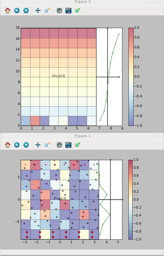
Note that these toy MD and CFD codes are provided as an example and there is no guarantee of the accuracy or correctness of either code. In fact, the constraint applied appears to need some work on the MD code.